Before we go into fully reinforcement learning, we first introduce a simpler model — K-armed Bandit Problem.

A K-armed Bandit Problem

You are faced repeatedly with a choice among k different options, or actions. After each choice you receive a numerical reward chosen from a stationary probability distribution that depends on the action you selected. Your objective is to maximize the expected total reward over some time period, for example, over 1000 action selections, or time steps.

Here you can imagine that you walk into a gambling house and see k bandit machines in front of you. They looks totally the same, but the amount of coins they are expected to spit is different, and you don’t know that expected values. Then you need to develop strategies to obtain the maximized reward. That’s the most tranditional bandit problem.

Here we give some notations:

$A_{t}$ : The action we select at time step t
$R_{t}$ : The reward of the action we select at time step t
$q_{*}(a)$ : The expected reward of action a
$Q_{t}(a)$ : The estimate reward of action a at time step t

$q_{*}(a) = \mathbb{E}[R_{t} | A_{t} = a]$

We would like $Q_{t}(a)$ to be close to $q_{*}(a)$.

Here we need to mention the most common problem in solving the problem — the trade off between exploration and exploitation. Why this? Supposed that you try multiple machines and find the one with the highest reward. One possible approach is that from now on you always select the optimal one. But there exist a problem that the bandit you choose is not the best, but only currently optimal. It means that there may exist some other bandits which have a higher expectation(mean value), but unfortunately behave bad in the first few trials(because the propability satisfies some distribution and has error). That’s why we need to explore more and try some other bandit.

Exploration here means the selection of nongreedy actions, while exploitation means the selection of that optimal actions. Exploitation is the right thing to do to maximize the expected reward on the one step, but exploration may produce the greater total reward in the long run.

In all, whether it is better to explore or exploit depends in a complex way on the precise values of the estimates, uncertainties, and the number of remaining steps. And we will also learn some simple algorithms and methods to balance between exploration and exploitation.

Sample Average

There are several ways to estimate the reward of a given action. One common method is sample average.

$Q_{t}(a) = \dfrac{sum~of~rewards~when~a~taken~prior~to~t}{number~of~times~a~taken~prior~to~t} =
\dfrac{\Sigma_{i=1}^{t-1}R_i\cdot\mathbb{1}_{A_i=a}}{\Sigma_{i=1}^{t-1}\mathbb{1}_{A_i=a}}$

And the simplest action selection rule is to select one of the actions with the highest estimated value(Greedy algorithm).

$A_t = arg_a maxQ_t(a)$

$\varepsilon$-greedy

As we mention above, we need to balance the exploration and exploitation. One simple approach is that we exploit greedily most of the time, but every once in a while, say with small probability $\varepsilon$, instead select randomly from among all the actions with equal probability, independently of the action-value estimates.

An advantage of these methods is that, in the limit as the number of steps increases, every action will be sampled an infinite number of times, thus ensuring that all the $Q_t(a)$ converge to $q_*(a)$.

Here we can compare the performance between these two algorithms.

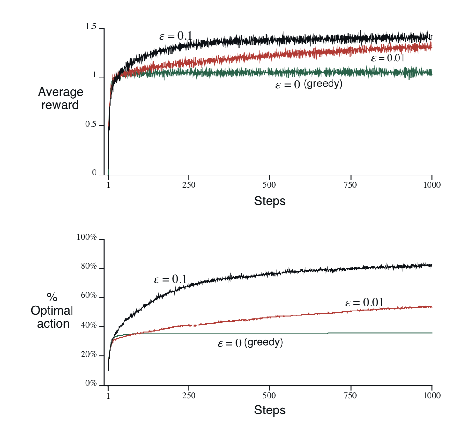
It is obvious that $\varepsilon$-greedy behaves better than greedy due to the simple balance between exploration and exploitation.

Nonstationary Problem

The averaging methods discussed so far are appropriate for stationary bandit problems, that is, for bandit problems in which the reward probabilities do not change over time. However, we will often encounter nonstationary problems. For example, the expected reward of bandits changes over time. In this case, the above algorithms will not suit anymore.

In nonstationary problem, we would like to focus more on recent rewards, instead of the total average rewards, as done in sample average. One of the most popular ways of doing this is to use a constant step-size parameter.

$Q_{n+1} = Q_n + \alpha[R_n - Q_n]$

By using a constant step-size $\alpha$ which is less than 1, each time an action is selected, the original reward(before update) is reduced by a fraction. It means that the weight given to $R_i$ decreases as the number of intervening rewards increases. This satisfies the idea we want — to focus more on recent reward. This method is also called exponential recency-weighted average.

Optimisitic Initial Values

All the methods we have discussed so far are dependent to some extent on the initial action-value estimate, $Q_1(a)$, let’s say they are biased by their initial values. However, this bias usually is not a problem, but instead can be very helpful.

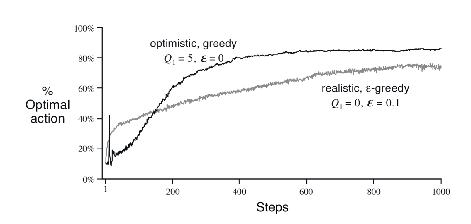
One common usage is to encourage exploration by setting a higher initial values. For example, instead of setting the initial values to 0, we can set them to +5, which is higher than $q_*(a)$. Then whichever action is selected, the reward is less than the starting estimates, and the learner switches to other actions. The result is that all actions are tried several times before the value estimates converge. The system does a fair exploration even if greedy actions are selected all the time.

Upper Confidence Bound

Before in $\varepsilon$-greedy, we randomly select among all actions every once in a while. However, this method has no preference for those that are nearly greedy or particularly uncertain. It would be better to select among the non-greedy actions according to their potential for actually being optimal, taking into account both how close their estimates are to being maximal and the uncertainties in those estimates. One effective way for doing this is as following:

$A_t = arg_a max[Q_t(a) + c \sqrt{\dfrac {\ln{t}} {N_t(a)} }]$

Here the square-root term is the measure of the uncertainty or variance of an action. If an action has been selected for many times, this term will be small and represents the true action-value estimate. If an action is seldomly selected, this term will be large and represents the upper bound of that action, which encourage the agent to explore.

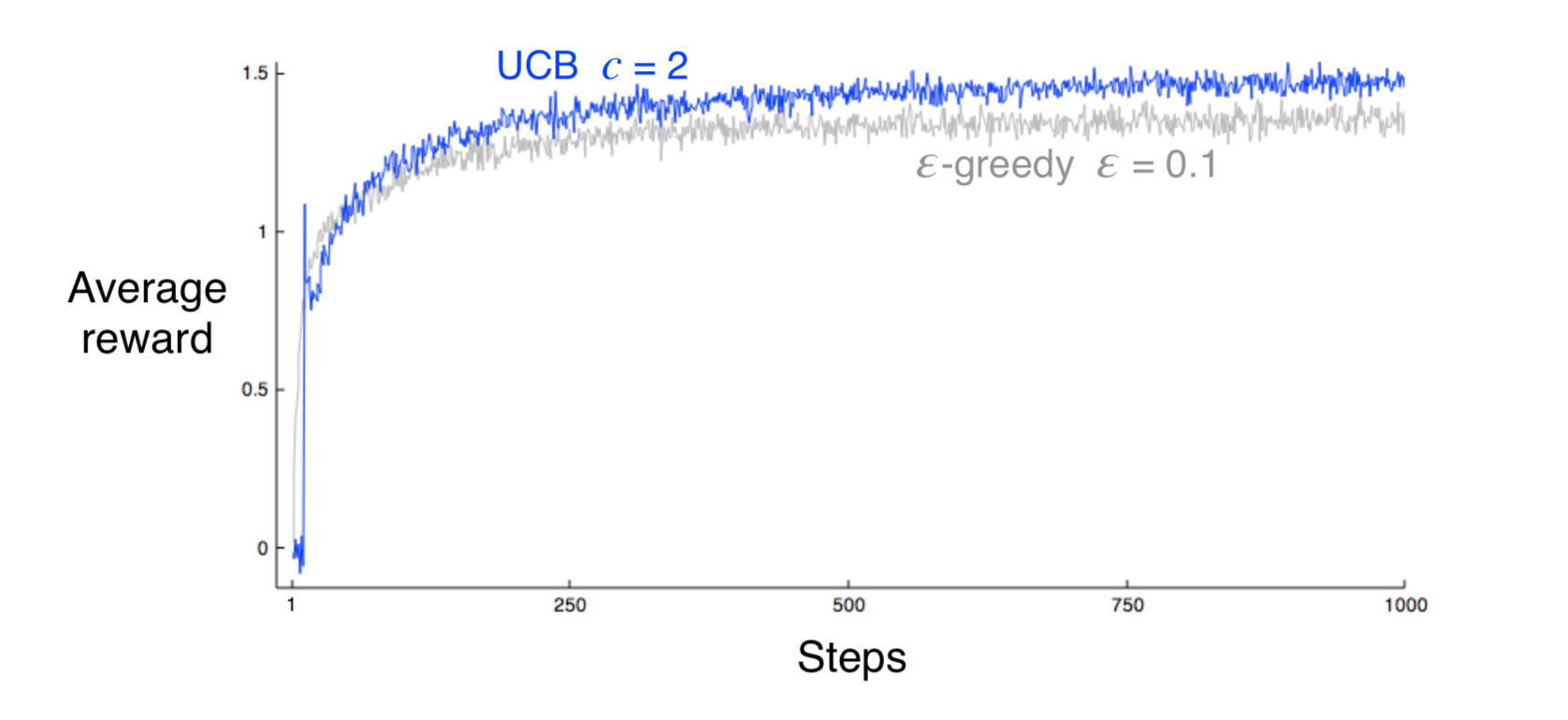
As we can see, UCB performs better than $\varepsilon$-greedy, but has some disavantages.

It cannot deal with nonstationary problem because the measure of uncertainty is not meaningful anymore.
It cannot deal with problems with large state spaces.

Gradient Bandits Problem

Instead of action value estimate, we can also learn a numerical preference for each action a, which we denote $H_t(a)$. The larger the preference, the more often that action is taken. The probability of selecting an action can be determined by a soft-max distribution as following:

$Pr\{A_t = a\} = \dfrac{e^{H_t(a)}} {\Sigma_{b=1}^k e^{H_t(b)}} = \pi_t(a)$

There is a natural learning algorithm for this setting based on the idea of stochastic gradient ascent. On each step, after selecting action $A_t$ and receiving the reward $R_t$, preferences are updated by:

$H_{t+1}(A_t) = H_t(A_t) + \alpha(R_t - \bar{R}_t)(1 - \pi_t(A_t))$

$H_{t+1}(A_t) = H_t(A_t) - \alpha(R_t - \bar{R}_t)\pi_t(A_t), \hspace{2cm} for~all~a\neq~A_t$

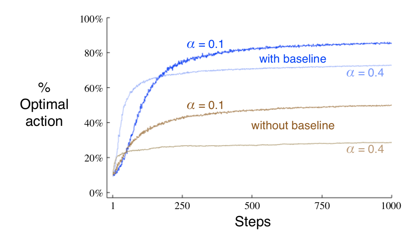
The $\bar{R}_t$ term serves as a baseline with which the reward is compared.

Associative Search

So far in this chapter we have considered only nonassociative tasks, that is, tasks in which there is no need to associate different actions with different situations. For example, in k-armed bandits problem, we only need to search for the optimal action without worrying the action we selected will affect the environment.

However, in a general reinforcement learning task there is more than one situation, and the goal is to learn a policy: a mapping from situations to the actions that are best in those situations. For example, in nonstationary bandit problem, now you will received a hint about their action values each time you select an action. The hint here can be the machine changes the color of its display as it changes its action value. Although you still have no idea the true action values, you can try to estimate the action values according to these hints. That’s the main target we would like to learn in reinforcement learning — the Policy.

Summary

In this chapter, we learn the simplest model of reinforcement learning — k-armed bandits problem, and also learn multiple useful methods to solve the problem. The $\varepsilon$-greedy methods choose randomly a small fraction of the time, whereas UCB methods choose deterministically but achieve exploration by subtly favoring at each step the actions that have so far received fewer samples. Gradient bandit algorithms estimate not action values, but action preferences, and favor the more preferred actions in a graded, probabilistic manner using a soft-max distribution. The simple expedient of initializing estimates optimistically causes even greedy methods to explore significantly.

We use a graph to compare their performance with different parameter settings.

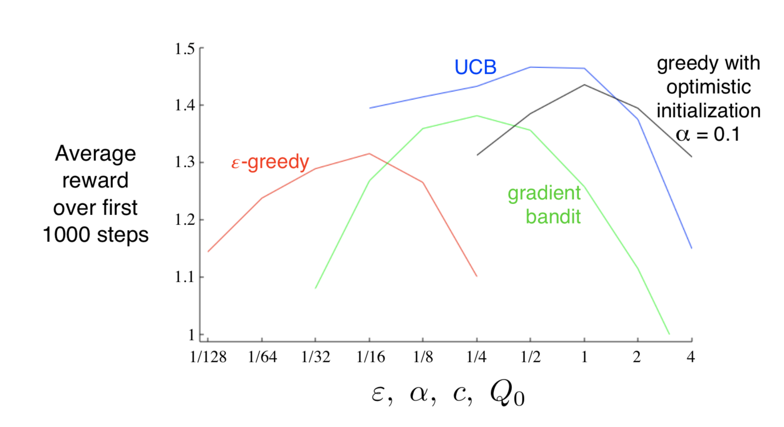
As we can see, all this methods are in inverted-U shapes, which means the parameter set for the method should be intermediate, not too large or too small. We can also observe that UCB performs the best among all these methods. To be true, we have some other sophisticated methods which is much more efficient in dealing with k-armed bandits problem, like Gittins or Bayesian, but their complexity and assumptions make them impractical for the full reinforcement learning problem that is our real focus.